The musical objects that are the focus of this book are fundamentally mechanical, which distinguishes them from objects in the world of music technology primarily defined by electronic circuits and computer programs. Mechanical aspects establish the affordances and constraints of systems in musical categories such as pitch range, speed, and dynamics. This chapter approaches mechanical topics from both theoretical and practical perspectives. It starts with definitions, concepts, and relationships in physics, such as between force, distance, and speed, which provide a foundation to the mechanical design process. A library of mechanisms is then introduced. It is likely that your design will require some kind of conversion, such as from linear to rotational motion; therefore, mechanisms will also be grouped according to scenarios where an input needs to be transformed to a different type of output. Methods for specifying key parameters for component selection, such as force and speed, will be reviewed, including mathematical calculations and modeling, research, and experimentation. The chapter concludes with an example that synthesizes these ideas. Like the other technical sections of this book, the following is not a comprehensive course of study in physics or mechanical engineering. Instead, it focuses on principles and mechanisms that are useful in the design of musical machines.
There are different kinds of motion. Translation refers to motion where every point on the object moves the same distance in a particular direction (e.g., a train). Rotation describes motion around at least one fixed point (e.g., a wheel). Reciprocation refers to motion that repeatedly moves up and down or back and forth (e.g., a piston). Oscillation is back and forth motion along an arc anchored at a pivot (e.g., a clock pendulum). These are shown in Figure 2.1.1.

A kinematic chain is an assemblage of linkages and joints that transforms an input motion into an output motion. A mechanism involves a kinematic chain that has been “grounded,” or attached to a frame of reference, transforming input forces and motion into a set of output forces and motion. A machine is an assemblage of objects that transforms forces, motion, and energy to do work (a mechanism doesn’t necessarily transform energy, thus the distinction between the two).
The study of mechanics has a number of sub-fields, which you may encounter or want to explore further. Dynamics is the study of forces and their effects on the motion of objects. Kinetics is the study of inertial forces in motion. Statics is the study of forces and their effects while machine parts are at rest. Kinematics is the study of motion without reference to the forces that cause such motion. In the next section, we will explore some of the principles from these fields in more depth.
Understanding the principles behind mathematical models of physical interactions allows you to conceptualize and quantify how parts of a system interact with each other. It can guide you when searching for related research and help you understand its findings. It can provide direction when designing and conducting your own experiments. There are theoretical concepts that, when understood, can help you implement the mechanisms that are most appropriate for a particular design.
Mass is a measure of the matter that constitutes an object. It is a fundamental quantity in all objects and plays a central role in the concepts and equations used in the design process. Mass and weight are not the same thing in physics, and the two terms are often confused. Weight (W) is the force of gravity on an object and can be calculated by multiplying the object’s mass (m) by the acceleration of gravity (g), which is 9.8 m/s² at the earth’s surface:
A 1-kg mass has a weight of 9.8 N on the surface of the earth.
Newton’s first law of motion states that a body in motion will tend to stay in motion and that a body at rest will tend to stay at rest. Inertia is the property of matter to stay in motion if already in motion, or at rest if already at rest. The inertia of an object depends on its mass: the more mass, the more inertia.
Sound is produced by the motion of physical objects. The motion of a musical machine or its parts may occur along a line, a circle, or some more complex path. Different types of motion are governed and described by specific sets of conceptual and mathematical principles. Linear (or translational) and rotational (or angular) motions are most common in musical machines, so we will focus on those.
The rate at which an object moves can be described in terms of velocity and acceleration. Velocity (v) describes the displacement (d) of an object over the period of time (t) of that displacement. Displacement and time are calculated by subtracting an initial value (i) from a final one (f). Average velocity (v) is determined by the following:
Acceleration (a) describes a change in velocity over a defined period of time (t):
Kinematic equations for linear motion. When we are trying to figure out a motion problem and know some of the variables but not another, kinematic equations can be of help. In these equations, v is velocity, v0 is initial velocity, a is acceleration, x is distance, and t is time. These formulas assume that acceleration is constant.
Δx = (v + v0)2 t
Δx = v0t + ½at2
v2 = v02 + 2aΔx
For example, if we wanted to determine the velocity of a linear drum actuator that started at rest and accelerated at 2 m/s² for 0.5 seconds (500 ms), the first equation could be used, yielding a velocity of 1 m/s. Velocity and acceleration are important in musical machines, as they are primary influences on sonic parameters such as dynamics.
Musical machines produce sound by exerting force on a sound-producing object. A force pushes or pulls on a body to change its acceleration. This change in acceleration affects how the body moves (e.g., rest → motion, speeding up, slowing down, changing direction). Force is a factor when striking a drum, fretting a string, or building the structure of an instrument. Newton’s second law of motion states that the acceleration of an object (a) is proportionally related to the force (F) acting on it and inversely proportional to its mass (m):
If the force on an object is constant, the more massive the object, the less it will accelerate (and vice versa).
Energy is required for a physical system to do work, and it is fundamentally associated with motion. Of the various types of energy, we are particularly interested in mechanical energy, which comes in two forms: potential energy (PE) and kinetic energy (KE).
Potential energy (PE) is stored based on an object’s position within a system, which can be used to do work or can be transformed into KE. Gravitational potential energy (PEgrav) is the energy that an object of mass (m) has as a result of its height (h) above earth, where g is the acceleration due to gravity (9.8 m/s²):
Example: A 0.005 kg marble held 1 m above a drum has 0.049 J of potential energy:
Elastic potential energy is the energy stored in materials as a result of their stretching or compressing. Many materials can store elastic potential energy, including rubber bands, membranes (e.g., a drumhead), and springs. The more these materials are stretched or compressed, the more potential energy they store. These objects are broadly useful, such as when returning an actuator (e.g., a solenoid) to its initial position after activation or offsetting the force of gravity.
A moving object has kinetic energy (KE), which is a function of its mass (m) and velocity (v):
Example: A drumstick with a mass of 0.05 kg that is traveling at 10 m/s has a KE of 2.5 J:
When the total energy in a system is the same before and after an interaction, energy is conserved. This is known as the law of the conservation of energy, which is represented as
where i indicates initial energy and f indicates final energy. In many cases, though, there is a loss of energy due to friction, heat, sound, and so on. This concept is important when we consider collisions between objects.
The conservation of energy (the total energy in a system is the same before and after an interaction) holds in transformations between inputs and outputs. The amount of energy that is conserved is expressed as efficiency (η), which is calculated as the ratio of energy output to energy input. If all energy is conserved, the system is 100% efficient, but in real-world examples, factors such as friction reduce the efficiency of machines.
In physics, work (W) is a measure of the transfer of energy when a force (F) is applied to an object over a distance (d) in the direction of the object’s displacement:
The unit for work is the joule (J).
Example: A force of 10 N applied to a drumstick over 0.5 m will produce 5 J of work.
The net work (Wnet) done on an object equals its change in kinetic energy (ΔKE), which is known as the work–energy theorem or principle. Using the earlier stated calculation for KE yields the following, where i is the initial value and f is the final value:
Substituting ΔKE for W in the work equation shows the relationship between an object’s change in kinetic energy (ΔKE), the average impact force acting on the object (F), and the distance the object traveled during impact / between impact and coming to a stop / deformation of an object (d):
The work–energy principle is useful for calculating the quantities involved in a collision, which are fundamental to producing sound.
We can describe a moving object as the product of its mass (m) and velocity (v), which is known as momentum (p):
The change in momentum of an object equals the product of the net external force acting on it and the time over which the force acts, which is known as the impulse of force:
Example: What force applied over 50 ms would be required to accelerate a drumstick with a mass of 0.05 kg from rest to a velocity of 10 m/s?
Like energy, the total momentum of a group of objects (a system) remains constant, which is known as the conservation of momentum. This means that the total momentum of a system is the same before and after interactions between its objects.
The concept of momentum allows us to describe the physical characteristics of an object as it moves, but how can we understand the quantities at work when that object collides with another object? Collisions are a way in which sound is made. In a collision between two objects, the force exerted on object 1 (F1) is the same in magnitude but opposite in direction to the force exerted on object 2 (F2). The time (t) of contact is the same for both objects, thus
As the product of force and time is equivalent to momentum change, we can rewrite the relationship in terms of mass (m) and velocity (v):
Fast forwarding through the mathematical proof, we see the equation for the conservation of momentum for two objects in a one-dimensional collision, which shows that the momentum of object 1 and object 2 before the collision (i) equals the momentum of object 1 and object 2 after the collision (f):
Example: A 0.01 kg ball collides with a 0.005 kg marble that is at rest. If the ball’s velocity before the collision is 17 m/s and 7 m/s after the collision, how fast will the marble travel?
v2f = (0.17 − .07).005 = 20 m/s
This kind of situation could be useful for making something Rube Goldberg–esque involving chain reactions that eventually produce sound (and many musical machines have been made that use marbles!).
Collisions can also be described in terms of energy. When KE is conserved, the collision is elastic. We can create an expression for the conservation of KE, as we did above with momentum, and solve the system using both equations (I will spare you this math, as it gets pretty hairy; the point here is to introduce the concepts at work). When all or most of the KE is dissipated (e.g., as sound or heat), the collision is inelastic. The elasticity of an object, its ability to return to its original shape after a deforming force is removed, varies given the properties of the material. We can account for the elasticity of an object mathematically using the coefficient of restitution (COR, denoted by e), which ranges from 0 (inelastic) to 1 (perfectly elastic). Musical collisions are typically partially inelastic, where some of the energy from the striker (e.g., the stick) is transferred to the sonic object (e.g., the drum) and some of it is converted into other forms, such as heat and sound. Not knowing the exact amount of energy transformed into other forms makes it difficult to specify the forces exerted on the drum membrane by a stick in motion. This brings us to a lesson when thinking about musical collisions:
Lesson: In the case of collisions, the variables that we can most directly manipulate that affect kinetic outcomes are the velocity and mass of the striking object.
Musical motions are often circular. A drummer’s arm rotates from her shoulder and elbow in the process of striking a drum. A pick follows an arc to bring it in contact with a string. The distances, velocities, accelerations, and forces involved are similar to their linear counterparts in some ways but conceptually and mathematically different in others. The following sections will review some of these similarities and differences.
When an object rotates around a point, we can calculate its displacement, velocity, and acceleration by using geometric concepts. In Figure 2.1.2, if an object travels from point 1 to point 2, the displacement of the object will be equal to the arc length separating the two points (S). Relative to the midpoint of the circle (the axis of rotation), the radius of the circle (r) moves, creating an angular displacement (Δθ), expressed in radians or degrees. That angle can be calculated by dividing the arc length by the radius:

Angular velocity is a measure of the rate of rotation of an object. Every point on a rotating object has the same angular velocity. Angular velocity (ω) can also be understood as the rate of change of an angle, which is calculated by dividing angular displacement (Δθ) by the time of the change (Δt):
The SI unit of angular velocity is radians / second, though rotational speed is also defined in revolutions per minute (RPM) and is indicated by the symbol N.
Angular velocity can be related to linear velocity. In the case of a circular path, linear velocity measures how the arc length changes over time. Linear velocity (v) is the distance traveled (s) divided by the time (t) of that travel. The distance (s) is rθ, so
Because ω = Δθ / t, the relationship between angular velocity and linear velocity is given as
This relationship shows that the instantaneous tangential velocity (Figure 2.1.3) of any point on a rotating object is proportional to the distance from the axis of rotation (the farther from the axis, the faster the velocity).

Angular acceleration (α) is the change in angular velocity (ω) over a period of time, expressed in rad/sec²:
When trying to figure out angular velocity, acceleration, or displacement, and some of the variables are known, but not others, the kinematic equations of rotational motion can be of help:
ω = ω0 + αt
θ = ω0t + ½αt2
ω2 = ω02 + 2αθ
where θ is angular displacement, ω is angular velocity, the subscript 0 indicates the initial value (e.g., ω0), α is angular acceleration, and t is time. Angular acceleration is assumed to be constant in these equations.
Angular velocity, acceleration, and displacement have significant effects on musical parameters, such as dynamic range.
Torque is a measure of force applied to an object that rotates around an axis. Torque can be static or dynamic. Static torque does not produce acceleration. Pushing the handle of a closed door is an example of static torque because the door doesn’t move. Dynamic torque produces angular acceleration, as when applying a force to a wheel to make it turn (thus, angular acceleration and torque are directly related). Torque is sometimes called moment or moment of force, and the distance between the point of rotation (axis, fulcrum, or center of mass) and the point where the force is applied is called the moment arm. Torque (τ) is a function of a force (F) applied to an object, the length of the moment arm (r), and the angle between the force vector and the moment arm (θ), as represented in Figure 2.1.4 and Equation 2.1.1:

When the force is applied at a 90° angle to the moment arm (as it is in Figure 2.1.4), then
The SI unit of torque is the Newton-meter, though the foot-pound is used as well.
We can think of Newton’s second law (F = ma) in terms of rotational motion: angular acceleration (α) takes the place of linear acceleration (a) and torque (τ) takes the place of force (F). As mass (m) is a measure of an object’s linear inertia, an object’s moment of inertia or rotational inertia (I) is a product of its mass (m) and the moment arm (r):
The SI units of rotational inertia are kg⋅m². Completing the analogy to Newton’s second law, in the case of a point mass (a theoretical object whose entire mass is located at a single point that is some radius from the axis of rotation), angular acceleration (α) is proportional to torque (τ) and inversely proportional to rotational inertia (I):
Given a constant torque, the larger the mass or the longer the moment arm, the lower the angular acceleration.
The rotational inertia of real objects (and not just point masses) becomes more complex. Real objects have different mass distributions that necessitate modifications to the above calculations. Rods are of particular interest in musical applications (e.g., drumsticks), and the rotational inertia (I) of a rod of length (L) with an axis at its end is
A rod rotating around an axis at its center (drumsticks don’t typically rotate from their ends) would be
A cylinder or disc rotating around an axis at its center, and a radius (r) would be
A sphere rotating around an axis at its center would be
The moments of inertia for a variety of objects are well-documented and can be found on the internet, so you can look up the equation for the object that you are incorporating into your design.
Rotating objects also have momentum, known as angular momentum (L), which is the product of the mass of the object (m), the velocity perpendicular to the radius (v⊥), and the distance between the axis and the object (r):
Conceptually, the important part of this relationship is that if the angular momentum and mass are constant, then reductions in the radius will result in increases in velocity.
For objects where the mass is distributed, such as a rod, angular momentum (L) equals the rotational inertia (I) times the angular velocity (ω):
This is the angular analog to the equation that describes linear momentum: p = mv.
Like momentum and energy, angular momentum is conserved. This means that if an object is spinning in a closed system and no external torques act on the object, it will continue to spin at the same rate. The conservation of angular momentum is exemplified by a spinning ice skater. As the skater pulls in her arms (creating a smaller moment arm), her rotational inertia decreases, so her angular velocity increases to conserve angular momentum (assuming little friction between her skates and the ice). As with linear movement, angular momentum is conserved when objects collide. This means that objects exert equal but opposite angular impulses on each other in a collision. Such aspects come into play when parts of a machine rotate, such as a drumstick on a pivot.
The basic physical principles described in the previous section help us better understand how work changes between inputs and outputs, which is a fundamental purpose of machines. Often, the available inputs do not produce the required outputs. You might have a motor that spins fast but doesn’t output enough torque. You might have an actuator that moves 3 centimeters, but the rod that is attached to it needs to move 1 meter. You might have a motor whose axle moves in a circle, but the fretter that it is connected to needs to move in a straight line. In all of these cases, mechanisms can transform the inputs you have into the outputs you need.
There are many mechanisms, ranging from simple to complex. Despite the shapes, sizes, and configurations of these objects, machines are generally used to achieve a limited number of goals, which include
- increasing or decreasing an input force.
- increasing or decreasing the distance over which that force is applied.
- increasing or decreasing the speed of an input.
- changing the direction of motion.
- transforming one form of motion into another form (e.g., linear to rotational).
There are relationships between these aspects that are essential to understand when dealing with mechanisms. There are trade-offs between force, distance, and speed, where increasing one quantity can decrease another (and vice versa), in both linear and rotational contexts. The primary relationships between physical aspects that come into play in the design of a musical machine are between force and distance, velocity and distance, and torque and speed.
A force can be manipulated by changing the distance over which it is applied. Because work is force (F) multiplied by distance (d) and energy is conserved between input and output (a machine cannot do more work than the work put into it), then
where the subscripts i and o indicate input and output, respectively. Mechanical advantage is a measure of the relationship between forces and distances between inputs and outputs. The ideal mechanical advantage (IMA) of a system equals the ratio of the output force (Fo) to the input force (Fi) or the input distance (di) to the output distance (do):
This relationship shows an inverse relationship between force and distance. Given a particular input force applied over a particular distance, an increase in output force occurs if that force is exerted over a smaller distance. In this case, the IMA of the system would be > 1. A decrease in output force occurs if it is applied over a longer distance, resulting in an IMA of < 1. This is important for musical machines because distance and velocity are related, as discussed next.
There is thus a trade-off between force and distance that must be balanced when choosing and designing a mechanism. There are many kinds of machines (including the six simple machines) that make use of this relationship. Note that these relationships are “ideal” because they assume there is no loss of work due to friction; in the real world, friction is common.
Linear velocity and distance are proportionally related, as average velocity (v) is a measure of the displacement (Δx) of an object over a period of time (Δt):
This means that, given the same period of time, velocity and distance are proportionally related:
If the output distance is twice the input distance and the time traveled by both is equal, then the output must be traveling at twice the speed of the input. This is one of the reasons to implement a machine with a mechanical advantage of < 1. The output force is less than the input force, but the output distance is greater than the input distance, which means the velocity of the output is greater than the velocity of the input. This principle is used in tennis rackets and golf clubs.
To illustrate the relationship between velocity and distance, imagine a rod rotating about a midpoint, as in Figure 2.1.5:

If the rod started in the position indicated by the brown line and then moved into the position indicated by the blue line, the outer part of the rod must travel at a greater linear velocity than the inner part of the rod, because it has to cover more distance in the same amount of time. Linear velocities thus vary depending on the distance between a point and the center of rotation. Note that we are assuming that the angular velocity, which is the rate of change of an angle (e.g., RPM), is constant in this case.
Understanding the relationship between torque and speed is important when designing musical machines, as motors are commonly used to generate movement. Torque is the rotational equivalent of linear force applied to a system, while speed, or angular velocity, is the rate at which the driven system rotates. The power of a rotating system is a product of the torque (τ) and angular velocity (ω):
Rearranging this equation shows that torque and angular velocity are inversely proportional:
Thus, given a constant power output, increases in torque are accompanied by decreases in angular velocity and vice versa.
The concepts in the preceding sections will help you understand how specific mechanisms work and why you would choose a particular mechanism for a design. The next step is to develop a library of devices that can be referenced to address specific problems and to inspire new ideas. While some sources differentiate between simple machines and more complex mechanisms that elaborate, transform, or combine them, they are conflated here as they are all building blocks that can be assembled within a design. As these examples are discussed, keep in mind that these mechanisms can produce sound, but they can also create physical movements and gestures that add visual interest to performance and define the identity of the machine (and its designer).
A lever uses distance to transform input and output forces. A lever consists of a straight, rigid object and a pivot point, called a fulcrum. The IMA is determined from the distance (Le) between the effort force (Fe) and the fulcrum (also known as the effort arm or input arm) and the distance (Lr) between the force exerted by the load (Fr) and the fulcrum (also known as the load arm or output arm), as seen in Figure 2.2.1:
Example: If Le is 4 cm and Lr is 1 cm, then the mechanical advantage of the lever is 4.
A lever is in equilibrium when the effort and the load balance each other:
Example: If Le is 3 cm, Lr is 1 cm, and Fr is 9 N, then the input force required to bring the lever into equilibrium is 3 N. The mechanical advantage of this system is 3.
There are three classes of levers, depending on the positions of the applied force, the fulcrum, and the load. In a first-class lever (Figure 2.2.1), the fulcrum is located between the applied force and the load. The mechanical advantage of first-class levers can be greater or less than one, depending on the position of the fulcrum relative to the effort force and the load.

In a second-class lever, the load is located between the applied force and the fulcrum, as in Figure 2.2.2.

Since mechanical advantage is the ratio of Le to Lr, second-class levers always have a mechanical advantage greater than 1. An example of a second-class lever is a wheelbarrow.
In a third-class lever, the applied force is located between the fulcrum and the load, as in Figure 2.2.3.

Here, the input force exceeds the output force, which means the mechanical advantage is less than one, but this enables increased control over the load. Tweezers, tongs, and the human forearm (the elbow acts as the fulcrum) are examples of third-class levers.
The distance that the load and the effort travel depends on the position of the fulcrum. As the lever moves, the load and the effort form a circular sector arc where the length of the arc (L) equals the angle of rotation (θ) multiplied by the radius (r):
Figure 2.2.4 visualizes these relationships where the distance from the load / output to the fulcrum is do, the distance from the effort / input force to the fulcrum is di, the distance traveled by the load / output is Do, and the distance traveled by the effort / input force is Di:

The angle θ is the same for both input and output, so
Di = θ × di
It follows that the ratio of the distance traveled by the output to the distance from the load to the fulcrum equals the ratio of the distance traveled by the input to the distance from the input force to the fulcrum:
Rearranging the equation, the ratio of the distance traveled of output and input equals the ratio of distance to the fulcrum of input / output:
All of this means that if the load arm is twice as long as the effort arm, then the load will travel twice the distance of the effort. Mechanical advantage is the inverse of this relationship as the ratio of the effort arm to the load arm, which in this case would be 0.5. An increase in output distance results in a decrease in output force. A decrease in output distance results in an increase in output force.
Levers are often used in musical machines. One common example is a drum-playing machine, which typically uses either a first- or third-class lever. In the case of a first-class lever, the fulcrum is located near the middle of the stick, the input force (e.g., via a push solenoid) is at the butt end of the stick, and the output force is at the tip of the stick, as in Figure 2.2.5.

The mechanical advantage of this system would be less than 1, given the proportions of the input distance to the output distance. Increasing the effort arm relative to the load arm would increase the mechanical advantage, and thus the output force exerted, but it would also reduce the distance traveled by the end of the drumstick and thus its linear velocity, which would affect the dynamic level produced.
Third-class levers are also common in machinic drummer designs, as seen in Figure 2.2.6.

As previously stated, this design would have a mechanical advantage of less than 1. As before, decreasing the effort / input arm (i.e., moving the solenoid closer to the fulcrum) will reduce the mechanical advantage of the lever and thus the output force, but it will increase the output distance traveled by the tip of the drumstick and thus its velocity.
In both cases, a balance must be struck between the required output force and the distance the tip of the stick travels. Larger output distances will allow the stick to accelerate for longer, reaching higher velocities that will affect the collision between the stick and the drumhead. Larger output distances create physical gestures that are more perceptible and engaging in performance, and help human musicians coordinate with their machinic collaborators. The trade-off is that larger distances take longer to travel, which can affect musical timing, and affect output forces, which may be a factor depending on what those forces are acting on. The challenge of the design is to find a configuration that achieves both sonic and visual goals.
A linkage is a body that connects to other components (including levers and other linkages) via joints. The joints allow the links to move by rotating or translating. Linkages can change the direction of motion (e.g., reverse motion linkages), transform force between inputs and outputs (e.g., parallel or push/pull linkages), or both (e.g., bell crank linkages), as seen in Figure 2.2.7.

Links can have different numbers of nodes that connect to other devices (e.g., a binary link has two nodes; a ternary link has three nodes). A series of connected links is called a kinematic chain. Any number of links can be connected to each other. A two-bar linkage consists of two links connected by a joint (e.g., pliers). A three-bar linkage won’t move, so it is a structure. Configuration and motion possibilities increase significantly with four links, so we will look at those devices in greater detail.
A four-bar linkage (Figure 2.2.8) has four links (a, b, g, f) that are connected by four rotating joints (A, B, C, D). Three of the links can move while the other is fixed in place (the ground link). A motor drives the input link, which forces the floating link (or coupler) and output link to move while the ground link stays in place.

A link that rotates fully is called a crank; a link that oscillates between two positions is called a rocker. The relative lengths of links will determine which are cranks and which are rockers, and a number of configurations are possible (e.g., crank-rocker, double-crank, double-rocker). Four-bar configurations produce varying output paths from a rotating or oscillating input (Figure 2.2.9). Transformations of motion are possible; for example, rotational motion can be converted to reciprocating motion (and vice versa). When the crank rod rotates, the rocker rod produces a reciprocating motion within a constrained angle.

There are several ways to integrate four-bar mechanisms into a design. One approach is to find an example that produces the desired motion and then scale the configuration accordingly. Another approach is to use software resources (such as mechanicalexpressions.com) that allow users to input linkage lengths and angular velocities to simulate the motions of different four-bar mechanisms. These tools allow you to determine a configuration that produces the desired path of motion. For example, Figure 2.2.10 shows a four-bar mechanism that produces a motion that could strike a chime (imagine the chime is located in point E’s path in Figure 2.2.10).
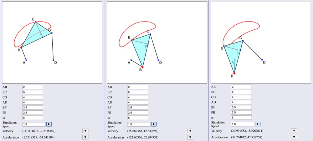
The characteristics of a four-bar mechanism can be calculated mathematically. The first step is to determine the mechanism’s dimensions and motions. Given the dimensions of a linkage and the angle of the crank, figuring out the position of the coupler is a forward (or direct) kinematics problem. Given the positions of the coupler, finding the link parameters that would enable motion through those positions would be an inverse kinematics problem. Finding the lengths and positions of the links is called linkage synthesis.
One approach to determining the lengths of the links and the position of the joints is graphical position synthesis (or the three-precision point linkage synthesis method):
- Represent the coupler in three different positions. Place points at one end of the coupler (blue).
- Draw lines (yellow) between the points.
- Draw equal-radius circles (dashed) around each point.
- Draw lines (red) through the intersections of the circles: these are the perpendicular bisectors of the lines (yellow) between the points.
- Extend the bisectors until they intersect. This is the center of the circle that passes through each point. This is the location of one of the pivots on the ground linkage.
- Repeat the process for the other end of the coupler, thus producing the location of the other pivot.
- Connect the links to produce the four-bar mechanism.
An important consideration is whether links will fully rotate (which can be problematic). The Grashof condition allows us to answer this question, which states that if the sum of the shortest and longest link is equal to or less than the sum of the remaining two links, the shortest link will be able to rotate fully. Let
L = length of the longest link
P and Q = the lengths of the other remaining links
If S + L ≤ P + Q is true, then at least one link will be able to rotate fully relative to the ground plane. If the inequality is false, then no link will be capable of a full revolution (Figure 2.2.11).

After determining the lengths of the links and the positions of the joints, prototype the design physically (e.g., using Legos, VEX components, cardboard, etc.) to get a sense of the system’s motion and reveal problems. Realizing a final design may require further specification of the system’s velocities, accelerations, and forces. While the mathematics involved in these analyses is outside the scope of this book, such approaches can help produce reliable performance and avoid the costs associated with trial and error.
The four-bar is the simplest of the closed-chain mechanisms. Greater numbers of links can be connected to make more complex mechanisms.
A slider-crank mechanism is similar to a four-bar linkage except that there is a slider instead of the output link (Figure 2.2.12). Because the slider moves along a track, the slider-crank mechanism is one option for converting rotary motion to linear motion. This device is useful when spanning relatively long linear distances. An advantage of the slider-crank is that it is highly configurable depending on the dimensions of the linkages. Potential disadvantages are that the input torque must be appropriately matched with the linkages so that they don’t break, and friction between linkages and between the slider and the track can cause wear and lower efficiency.

The slider-crank mechanism has numerous musical applications. It could be used as a fretter that travels along the neck of a string instrument to produce different pitches (as in Animusic’s Resonant Chamber). It could be used to power a string instrument’s picking mechanism. It could be attached to a trombone slide. One of the primary advantages of the slider-crank mechanism in artistic contexts is that its form and motion are visually apparent, which can help define the identity of an instrument and make it more compelling to watch in performance.
An eccentric-and-rod mechanism contains a circular disc (sheave) that is fixed to a rotating axle offset from the disc center (Figure 2.2.13). The sheave rotates within a housing (strap) that is rigidly connected to a rod. As the axle rotates, the sheave turns with it. The offset of the axle from the center of the sheave causes the attached rod to move forward and backward. The mechanism is thus capable of transforming rotational motion into reciprocating motion. Eccentrics produce high amounts of friction and thus are not typically used to transmit large forces.

A treadle linkage can convert rotary motion into reciprocating or oscillating motion, and vice versa. The mechanism involves a wheel connected to a linkage, which in turn is connected to another linkage, fixed at a pivot point (Figure 2.2.14).

Treadle mechanisms have a long history and are particularly significant in musical machines before the twentieth century. Foot-operated treadles were commonly used in player pianos and pianolas to operate the bellows that regulated air pressure in the instruments.
The wheel and axle is a simple machine that comprises a circular disc (wheel) with a rod attached to the middle of it (axle) that can be used to move a load (Figure 2.2.15).

Like the lever, the wheel and axle works by creating a longer distance over which a smaller input force is applied (to the wheel) relative to the larger force output over a smaller distance (by the axle). The work (F × d) done at the input and output must be equivalent because of the law of conservation of energy. The IMA of a wheel and axle is calculated by dividing the radius of the wheel (R) by the radius of the axle (r):
A wheel and axle has many musical applications. It could tension a string by attaching the string to the axle and then turning the wheel, which would wrap the string around the axle. It could be the basis for a picking or plucking device. If plucking objects (e.g., picks) are placed around the circumference of an axle, turning the wheel brings them in contact with the string. Alternatively, the plucking objects could be attached to the circumference of the wheel, driven by the rotation of the axle (note, if applying effort to the axle, IMA < 1). This is a common design seen in robotic string instruments, including GuitarBot (Singer et al., 2003), MechBass (McVay et al., 2011), and EMMI / MPR Lab’s PAM (Figure 2.2.16).

A gear is a wheel with teeth. The teeth allow gears of different sizes to interface, forming a gear train that increases or decreases the speed and torque of a rotating input. In addition, they can move rotational motion to a different axis, synchronize the rotation of two axes, and reverse the direction of rotation (meshed gears in a gear train always turn in opposite directions). The mechanical advantage of a gear train is a function of the gear ratio (GR), which is the ratio of the angular velocity ω of the input gear (in) to the angular velocity of the output gear (out). The gear ratio can also be expressed in terms of the gear’s radius (r) and number of teeth (N):
In an ideal gear train, gear ratio equals the mechanical advantage (MA), which is the ratio of output force to input force. This means there is an inverse relationship between force and angular velocity. For example, if input gear I has a radius of 1 inch and output gear O has a radius of 2 inches, the gear ratio would be 2:1. This means that the force output by gear O would be twice that input to gear I, but gear I would rotate at twice the speed of gear O. Similarly, if gear I has 25 teeth and gear O has 50 teeth, then the gear ratio between them would also be 2:1 (Figure 2.2.17), and the same relationship between angular velocity and force would exist.

Combinations of different-sized gears within a gear train allow increases or reductions in rotational speed and torque as desired. For example, given a 2:1 ratio between gear O and I as previously described, a desired output speed of 100 rpm at gear O could be achieved by rotating gear I at 200 rpm. An easy way to determine output speed is by dividing input speed by the gear ratio:
Gears that are meshed will turn in opposite directions. To move the drive and driven gears in the same direction with parallel shafts and without changing the gear ratio, an idler gear can be used, as shown in Figure 2.2.18.

Spur gears are common, with teeth that are straight and parallel to the shaft axis (Figure 2.2.17). Cons of spur gears include tooth contact that can produce noise and wear.
Helical gears have teeth that are angled relative to the direction of the shaft (Figure 2.2.19). This tooth orientation means they engage with each other more gradually as the shaft rotates, making the interaction between parts smoother and reducing noise. The downsides of the increased contact between the teeth are lower efficiency and the need for lubrication. Helical gears generate a large amount of thrust (a force acting parallel to the axle) that can be mitigated by thrust bearings. Helical gears are often more expensive than spur gears.

Bevel gears are mounted on shafts that are perpendicular to each other (though other angles are possible), which is handy when an input (such as a motor) and an output (such as a wheel) cannot be configured in a straight line (Figure 2.2.20). The teeth of bevel gears can be straight (like in spur gears), spiral (like helical gears), or hypoid (which can engage with axes on different planes). Advantages of bevel gears are that they are quiet, have increased torque capacity, and have high efficiency. Disadvantages are that they must be positioned precisely, have limited gear ratios, and are expensive.

A worm gear has a threaded shaft (worm) that interfaces with a gear’s teeth (worm wheel). When the shaft completes one complete revolution, the gear advances one tooth. The number of teeth on the gear determines the gear ratio (e.g., a gear with 25 teeth would have a 25:1 gear ratio). Worm gears are particularly useful because they can prevent backdriving, where the gear drives the shaft. Consider a guitar tuning machine, which incorporates a worm gear (Figure 2.2.21). Rotating the knob (or button) turns the shaft, which turns the gear, which turns the tuning post that the string is attached to, which is tightened or loosened. When the knob is released, the string’s tension drives the gear, which in turn drives the shaft. A worm gear can be designed so that torque applied to the gear shaft creates internal friction, which causes the mesh (the engagement of the gear and shaft) to lock, thus reducing or eliminating backdriving. The brilliance of this design is that once the desired position has been reached, no other force needs to be applied to keep it there. For example, using a motor to directly tension a string requires continuous application of torque (which requires power), even after the desired pitch is achieved. With a worm gear, the motor can drive the tuning machine to the desired pitch and then can be turned off: the worm gear holds the string at that tension without further power consumption.

Spur gear trains are oriented side-by-side so that each gear rotates about its own axis (e.g., Figure 2.2.18). In some cases, it is preferable to have only one axis of rotation, in which case a planetary gear system can be used. In a planetary gearbox (Figure 2.2.22), input and output shafts are aligned, which minimizes the device’s form factor. Planetary gears are typically used to reduce speed and increase torque. A planetary gear set includes
- A gear at the center (the sun)
- Multiple planet gears that surround the sun
- The ring, or outer gear, that surrounds the planets
- The carrier, which connects the centers of the planet gears to ensure proper meshing

The sun, planet, or ring gears can be the input, output, or can be stationary. For example, the sun gear could take a high-speed, low-torque input and drive the surrounding planet gears and ring gear. The carrier is connected to the planet gears, which can be used to drive an external load at the higher torques produced through the gear train. Planetary gears are highly efficient, compact, offer a wide range of gear ratios, and are precise. Their disadvantages are that they are complex and require precise manufacturing, making them expensive.
Rack and pinion gears translate rotational motion into linear motion. As the pinion gear turns, its teeth engage with those on the rack, which subsequently moves left or right depending on the direction the pinion turns (Figure 2.2.23).

While straight gear racks and pinion systems were known for friction and wear, helical systems have improved efficiency and are capable of smooth, quiet operation. Longevity is increased with proper lubrication. This kind of system could be useful if you need to make small linear adjustments. For example, imagine you want to change a string’s tension. By coupling a motor to the pinion gear and fixing one end of a string to the rack (the other end of the string must be anchored), turning the motor can increase or decrease the string’s tension.
A pulley is a wheel over which a rope, belt, or cable is passed to transmit motion (Figure 2.2.24). A pulley reduces the input force needed to produce an output force by increasing the distance over which the input force is applied. A pulley can also change the direction of a force (e.g., pulling down on a rope wrapped around a pulley to lift a piano to a second story). The IMA of a pulley depends on the number of rope segments supporting the load (N):
In Figure 2.2.24, the pulley on the left has an IMA of 1, while the pulley on the right has an IMA of 2. This means that the pulley on the right would require half the force as the pulley on the left, but that force would have to be exerted over twice the distance.

Pulleys and gears are the basis for mechanical drives, which transmit power (velocity and torque) from prime movers (driver shaft) to machine parts (driven shaft), convey materials from one location to another, and synchronize movements between systems. Three kinds of mechanical drives are useful in the case of musical machines: gear, belt, and chain.
Belt and chain drives transmit power from one component to another. These systems consist of a loop of material that runs over and connects multiple pulleys. In a belt drive, power is transmitted through friction between the belt, typically made of plastic or rubber, and the wheels. In other cases, the loop and the wheel engage. The teeth of a timing belt mesh with those of a sprocket (a toothed wheel) to ensure the movements of system components are synchronized (e.g., the camshaft and crankshaft in a car’s engine). In a chain drive, the drive chain (roller chain, transmission chain) passes over a sprocket so that the teeth of the sprocket mesh with the spaces in the links of the chain (Figure 2.2.25).

Drives typically have at least two gears. In some cases, a tensioner removes slack in the belt (Figure 2.2.26). Idler gears (Figure 2.2.18) can change the direction of rotation of the output shaft without affecting the gear ratio of the system.

Drives can increase or decrease the speed between an input and an output. Like gears, the bigger the wheel, the slower it turns. The velocity ratio between two pulleys is determined by the ratio of their diameters:
The output speed can then be determined by the input speed and the velocity ratio:
Example: Input pulley I has a diameter of 3.5 inches and is rotating at 100 rpm. If output pulley O has a diameter of 7 inches, how fast is it rotating?
Mechanical drive types have unique advantages and disadvantages. Chain drives are durable when made of metal and don’t slip (like belt drives). They produce constant angular velocity (unlike belt drives), and they are highly efficient (up to 98%). Conversely, they make noise, require lubrication, and are usually best suited for smaller distances (roughly 3 meters). Belt drives are simple to use and can be quieter, cleaner, smoother, and more cost effective than chain drives (particularly for longer distances). Conversely, belt drives are often not as durable, as they can stretch and snap. They can also slip if there isn’t enough friction between the belt and the wheel, or if they are not tensioned appropriately. The increased tension on the belt increases the load on the shafts and bearings. The possibility of slippage means that belt drives may not be appropriate for heavy transmission applications. Environmental conditions may affect belt drives more than chain drives. Gear drives can produce constant velocity ratios, can transmit large amounts of power efficiently, are durable, and are compact. The disadvantages include that they can be noisy, they cost more than belt and chain drives, and they require regular lubrication. These differences are reflected in Table 2.2.1.
| Belt | Chain | Gear | |
|---|---|---|---|
| Speed / torque | High speed, low torque | Low speed, high torque | Variable; can achieve high torque |
| Load capacity | Less | Good | Best |
| Distance | Short–long | Short | Short |
| Velocity | 12–40 m/s | <10 m/s | Varies with the type of gear |
| Constant velocity | No (flat belts) | Slight fluctuations | Yes |
| Durability | Less | Good | Best |
| Noise | Low | High | Variable |
| Environmental conditions | More sensitive | Resilient | Resilient |
| Maintenance | Tensioning, replacement | Lubrication, slack | Lubrication, cooling |
| Geometric flexibility | High | Lower | Lower |
| Slip / creep | Yes | No | No |
| Efficiency | Good | Better | Best |
A screw consists of an inclined plane wrapped around a cylinder. It converts rotational motion into linear motion. The pitch of a screw is the axial distance (parallel to the screw’s axis) between the screw threads (Figure 2.2.27). The lead is the axial distance traveled by the thread during one full revolution of the screw.

The mechanical advantage of a screw is the ratio of the distance the effort moves (DE) to the distance the load moves (DR). The distance of the effort is the circumference of the circle over which the force is applied (2πr). For example, if the screw was turned by hand, then the circumference would equal the head of the screw. The distance the load moves is the lead (l):
Screws are identified by their diameter and threads / inch:
- ½–14 means that the screw has a diameter of ½ inch, there are 14 threads / inch.
- 8-32 means that the screw has a diameter of less than ¼ inch and is thus indicated by trade number (#8, lower numbers mean smaller diameters), and there are 32 threads / inch.
- M5 indicates the screw diameter is 5 mm.
Screws are used as fasteners, but they can also be used to amplify force according to the above parameters.
A lead screw consists of a threaded rod, the screw, and a nut in contact with the screw. If the nut is constrained, rotating the screw will cause the nut to move forward or backward along the screw’s threads (Figure 2.2.28). The lead screw transforms rotational motion into linear motion.

The lead screw has a large mechanical advantage and can move large loads, is simple, smooth, quiet, the direction of travel is reversible, is suitable for vertical configurations, is relatively less expensive (than ball screws), and is self-locking without a braking system (it cannot be backdriven). Conversely, they produce significant friction, so they are not particularly efficient; they require greater input torque and their threads can wear. They are not as well-suited for high-speed applications. Lead screws have many applications in musical machines, such as a moving bridge for a string instrument and as a dynamic tensioner for a drum membrane.
A ball screw is similar to a lead screw except that it uses ball bearings to reduce the friction between the screw and the nut, which have matching helical grooves (Figure 2.2.29).

The advantages of ball screws are that they have lower friction and are more efficient, requiring less torque, running at cooler temperatures, and offering greater longevity. They can carry heavier loads than lead screws. The disadvantages of ball screws are that they are noisy, expensive (relative to lead screws), require braking systems to prevent backdriving, can be problematic in vertical configurations, and require lubrication. Ball screws typically cannot accelerate or maintain the same speeds as rack and pinion mechanisms.
Cam mechanisms transform rotational motion into linear motion. The essential parts of the mechanism are the cam, camshaft, crank, and follower. As the cam turns, the follower’s position changes depending on the cam’s shape. Different cam shapes yield different follower motions, enabling a simple rotational input to be transformed into more complex output motions. The resulting motion depends on the cam and follower shapes and their interaction. Common shapes for cams include circular, pear, snail / drop, and heart-shaped / constant velocity (Figure 2.2.30). The follower can produce linear / translational or oscillating motion. Follower designs include the knife-edge, roller, and flat face.

Advantages to cam and follower mechanisms include being able to produce a wide variety of motions in a simple and (potentially) compact way. Disadvantages include friction and backlash between the cam and follower, larger ranges of motion require larger cams, and they must be manufactured precisely.
The other simple machines (the inclined plane and wedge) are less common in the world of musical machines but will be described briefly in case they may be of some use. An inclined plane is just what it sounds like (Figure 2.2.31), and its mechanical advantage is determined by the ratio of the length of the incline (L) to the vertical rise (h):

Significant friction between the load and the plane can reduce efficiency, which can be addressed through a rolling device. A wedge drives objects apart (e.g., a log splitter). It gains mechanical advantage from the relationship between the wedge’s depth of penetration and the separation of the wedged surfaces. There aren’t many examples of musical machines that make use of inclined planes and wedges, but they are possibilities for the creatively adventurous.
The machines described can be combined to form more elaborate structures that modify forces, distances, and speeds. For example, a can opener or shovel (wedge and a lever), an exercise machine (levers and pulleys), a car jack (lever and screw), and a bicycle (wheel and axle and pulley) all combine the advantages of different machines. Musical machines, particularly those of the pre-twentieth century, also make use of combining mechanisms. The player piano of the early twentieth century and Wintergatan’s Marble Machine are prominent examples from the more recent past. These more complex mechanisms become necessary as musical requirements become increasingly sophisticated, such as increasing dynamic range or damping vibrating elements. The details of these systems are considered in greater depth in the Percussion, Strings, and Aerophones chapters of the book.
A spring is an elastic object that stores and releases energy. A spring doesn’t transform forces in the way that other mechanisms do. Instead, a load applied to a spring causes it to deform. The energy from this deformation is stored and is subsequently released as the load is removed from the spring. The distance (x) that a spring stretches or compresses depends on the force (Fs) applied to it and the spring constant (k) or the spring rate, which is a measure of the spring’s stiffness. The spring constant is dependent on the diameter of the wire, the diameter of each coil, the length of the spring at rest (free length), and the number of coils. The relationship between force, distance, and spring constant is represented in Hooke’s law:
Example: A 5 N block compresses a spring 0.05 m. What is the spring constant?
Hooke’s law can also be stated in terms of the restoring force of the spring (the force exerted by the spring back on the object compressing or stretching it), which is exerted in the opposite direction of the displacement (hence the negative sign):
Both of these equations are useful when specifying a spring for an actuating system: the actuator needs to produce enough force to compress the spring (F = kx), and the restoring force returns the system to equilibrium (F = −kx).
There are many kinds of springs; the most common include compression, extension, and torsion springs. Relevant dimensions include:
- Inside diameter (ID)
- Outside diameter (OD)
- Wire diameter
- Free length
Performance parameters include:
- Spring rate (the amount of force required for every inch or millimeter of compression)
- Compressed length at maximum load (solid length)
- Deflection (the distance traveled after full compression)
- Total coils
- Material
Compression springs are helical coils of wire that provide an opposing force when compressed. In addition to the standard parameters mentioned above, compression springs are specified by their ends, which are either open (left as cut) or closed (flattened to create more of a square end). Extension springs are helical coils of wire that provide an opposing force when stretched. In addition to the standard parameters, extension springs are specified by their length of body coils, length inside hooks (no load), and hook type. Torsion springs are helical (spiral) or flat coils or strips that are used to provide an angular force in response to a source of torque. In addition to the standard parameters, torsion springs are specified by wind direction and leg length. There are many other types of springs, including disc, strip, and rotor (Figure 2.2.32).

- McVay, J., Carnegie, D. A., Murphy, J. W., & Kapur, A. (2011). Mechbass: A systems overview of a new four-stringed robotic bass guitar. Proceedings of the 19th Electronics New Zealand Conference (ENZCon), Dunedin, New Zealand, 145–150.
- Singer, E., Larke, K., & Bianciardi, D. (2003). LEMUR GuitarBot: MIDI robotic string instrument. Proceedings of the International Conference on New Interfaces for Musical Expression, 188–191.
You will likely find yourself with an input that acts in one way when you need an output that acts in another. You may not know which mechanism can produce the conversion you need, or you might want to weigh the pros and cons of different options. It is therefore useful to group mechanisms by the types of conversions they accomplish (which is more convenient than reviewing each mechanism’s description to see if it might work). This section provides a quick reference you can check when you want a sense of mechanisms that might work for your situation.
A common scenario is that the motion of an input device is rotary when the desired motion of the output is linear (or vice versa). For example, imagine that you want to make a machine that plays the drums. Typically, a drumstick follows a circular (or at least pseudo-circular) path as it moves. If you have a linear actuator, such as a solenoid, you need a mechanism to convert the linear input motion into the rotational motion required. Conversely, you might have a DC motor whose shaft rotates when the output motion that is needed is linear. The following are mechanisms that convert rotation to translation:
- lead screw
- ball screw
- rack and pinion
- slider-crank
- cam and follower
- belt drive
- chain drive
Several devices convert rotary motion to oscillating motion and vice versa. These mechanisms allow you to use a rotary input, such as a DC motor, to produce oscillating motion to perform musical actions such as striking a drum or picking a string. The following mechanisms convert rotation to oscillation:
- treadle linkage
- four-bar
- peg / slot linkage
- cam and follower
The amount of force that is produced by a machine affects musical characteristics such as dynamic range, articulation, and timbral quality. Often, an input force needs to be increased or decreased to achieve a particular musical goal. The following mechanisms increase force between input and output:
- first-class lever with an effort arm that is > the load arm
- second-class lever
- wheel and axle where the effort is applied to the larger radius
- gear train where the
- angular velocity of the input gear > angular velocity of the output gear
- radius of the input gear < radius of the output gear
- number of teeth of the input gear < number of teeth of the output gear
- pulleys
- screw
- linkages
The following mechanisms decrease the force between input and output:
- first-class lever with an effort arm that is < the load arm
- third-class lever
- wheel and axle, where the effort is applied to the smaller radius
- gear train where
- angular velocity of the input gear < angular velocity of the output gear
- radius of the input gear > radius of the output gear
- number of teeth of the input gear > number of teeth of the output gear
- linkages
When output force is less than input force, the output will travel a greater linear distance than the input in the same amount of time, thus the output will move at a greater speed. For rotary motion, torque and angular velocity are inversely proportional. Based on these principles, the following mechanisms can be used to increase the speed of an output:
- first-class lever with an effort arm that is < the load arm
- third-class lever
- wheel and axle, where the effort is applied to the smaller radius
- gear train where
- radius of the input gear > radius of the output gear
- number of teeth of the input gear > number of teeth of the output gear
- mechanical drive where the diameter of the driven pulley is < the diameter of the driver pulley
- linkages (depending on the configuration)
Mechanisms that can reduce the speed of an input include:
- first-class lever with an effort arm that is > the load arm
- second-class lever
- wheel and axle where the effort is applied to the larger radius
- gear train where the
- radius of the input gear < radius of the output gear
- number of teeth of the input gear < number of teeth of the output gear
- mechanical drive where the diameter of the driven pulley > the diameter of the driver pulley
- linkages (depending on the configuration)
In many scenarios, the source of an input force must (or should) be physically distanced from the parts that are being driven by that input. Mechanisms that can transmit forces include:
- chain and belt drives
- Bowden cables (which contain an inner cable within an exterior housing)
In some cases, the direction of a force must be changed. The following mechanisms are capable of these conversions:
- idler gears
- pulleys
- linkages (e.g., reverse motion, bell crank)
The following table summarizes the advantages and disadvantages of different mechanisms. Note that performance within any of these categories can vary widely depending on the mechanism’s design and manufacture; for example, some rack-and-pinion systems exhibit significant friction, while others exhibit considerably less. With that said, an understanding of the strengths and weaknesses of mechanism categories is useful in the design process, as summarized in Table 2.3.1.
| Mechanism | Pros | Cons |
|---|---|---|
| Lead screw |
|
|
| Ball screw |
|
|
| Rack and pinion |
|
|
| Slider-crank |
|
|
| Cam and follower |
|
|
| Belt drive |
|
|
| Chain drive |
|
|
| Spur gears |
|
|
| Helical gears |
|
|
| Planetary gears |
|
|
| Worm gears |
|
|
With knowledge of different types of mechanisms and their capabilities established, realizing more complex machines requires putting simpler components together. There are many options for doing so, and the right one depends on the situation. Will the connection form a rigid body, or will it allow motion? If it is to allow motion, what kind? What kind of friction will result from this motion? What forces will be applied to the connection? Asking these basic questions will allow you to choose the right device. Brackets, joints, shafts, and bearings are particularly useful in these efforts.
Brackets connect two objects so that they form a rigid body. Some examples of brackets are seen in Figure 2.3.1: flat surface brackets connect surfaces at a corner (a) or in a “T” configuration (b), corner brackets connect objects from the interior at a 90° angle (c), and offset-surface brackets (d) connect two objects in a way where the surfaces are parallel but displaced relative to each other. Often these brackets are attached with screws or bolts. Specialized brackets are available for T-slotted aluminum (e.g., from McMaster-Carr or 80/20), which can be moved and removed within the bar’s interior channels to allow for experimentation and modification. When satisfied with dimensions and configuration, welding provides the surest connection, but it is a commitment that should be entered with full conviction.

A joint connects links and, in doing so, both permits and constrains motion. Joints are classified according to the motion, contact, and closure between components, as well as the number of links that are connected. Different types of joints include
- universal (has an angular range from 90° to 270°)
- ball / spherical (turns and swivels)
- screw
- pin / revolute (turn about a fixed axis)
- cylindrical (sliding and rotation)
- sliding / prismatic
- planar (flat)
as seen in Figure 2.3.2.

Some designs may call for a specific joint type, and others may accommodate a range of possibilities. In these cases, try candidates out and weigh the pros and cons: Does the joint allow the motion desired? How much friction or noise does it produce? How easy is it to implement, and how robust is it? How does it fit with the visual aesthetics of the design? The process may inspire new ideas for how the machine can move, enhancing its sonic or visual interest.
Shafts can be connected with couplers. Determine the diameters of the two shafts (if they are different, an adapter can be used), the shaft type (e.g., round, keyed, hex, spline, square; Figure 2.3.3), and whether the coupler needs to be flexible or rigid. Couplers can be purchased (e.g., from McMaster-Carr) or can be made. Couplers hold shafts in place using different methods. A common design uses set screws, which are tightened to keep the shaft in place (Figure 2.3.3, f). The problem with set screws is that, over time, they can loosen, causing backlash or slop in the system, reducing precision. Set screws can also mar the shaft. One solution to these issues is a clamping shaft coupling, which grips evenly around a shaft to provide more holding power (Figure 2.3.3, g). Another is a keyless bushing (e.g., Fenner Drives B-LOC and Trantorque), which uses the wedge principle and a single locking nut, respectively, to provide zero-backlash mountings.

Mounting hubs (Figure 2.3.4, left) affix to a shaft using a set screw, providing a flat plate for coupling to other objects (such as a pickwheel for a string instrument). Hose clamps (Figure 2.3.4, right) allow you to secure objects to a cylinder. They are also useful as a “stopper” to constrain the movement of cylinders or objects threaded through them: we use them on rod-mounted modular percussion units and on PVC tubes.

Motion between two objects in contact causes friction, which converts energy into noise, heat, and wear. These are usually not desirable and can be mitigated by friction-reducing components such as bearings. Axial bearings withstand force in the same direction as the shaft. Radial bearings withstand force perpendicular to the shaft.
There are many kinds of bearings, including plain, rolling, ball, thrust, and linear. A plain bearing (slide bearing, sleeve bearing, bushing; Figure 2.3.5, a) consists of only a smooth bearing surface that reduces friction between it and the journal (e.g., the part of the shaft that is mounted in the bearing). It has no rolling elements and thus is the simplest type of bearing. The sleeve of a plain bearing usually consists of soft metal or plastic and a lubricant to reduce friction. Plain bearings allow for linear, rotary, oscillatory, or reciprocating motion. They are simple, quiet, inexpensive, compact, and lightweight, and can withstand heavy loads. Rolling bearings contain balls or cylinders that reduce the friction between moving surfaces. Ball bearings are common (Figure 2.3.5, b), which contain a rolling element (steel balls connected by a cage) that separates a moving inner sleeve connected to the journal and a stationary outer sleeve seated in a housing (e.g., a flange or a structural component). Ball bearings can handle radial and axial loads but have limited load capacity. Roller bearings contain cylindrical elements instead of balls and can tolerate higher loads. Thrust bearings (Figure 2.3.5, c) are specifically designed to withstand axial loads. Linear bearings (Figure 2.3.5, d) facilitate motion along a straight path and can be ball- or roller-type. Linear bearings are useful in many musical situations, such as when moving a fretting carriage along the length of a string instrument. Magnetic bearings replace the ball or rolling elements with magnetic ones, thus removing moving parts and friction. They are particularly well-suited for high-speed and low-noise applications. Reducing friction is particularly important in musical machines because friction depletes the energy transferred from input to output, results in wear, and produces noise.

Physical quantities such as force and velocity need to be defined to produce a mechanical design that works as expected. How fast does a motor need to rotate? How much torque does it need to output? How fast does a drumstick need to move and over what distance to produce the dynamic range desired? There are several approaches that can be used to address these questions, each with pros and cons, including trial and error, research, calculation and modeling, and experiment.
Trial and error can be the (seeming) path of least resistance. It doesn’t require knowledge of complicated physical principles or mathematics, or extensive research through a body of publications. It allows you to escape the machinations of theorizing and get to the action. Calculations often represent ideal scenarios rather than the real-world ones that involve machining tolerances and friction. The trial-and-error method allows you to get your hands on physical parts, which can help you understand what is elusive in mental or representational domains. It allows you to approach the design and realization process iteratively (hopefully), learning and improving with each step.
Trial-and-error has drawbacks. The most significant of these is that it is expensive in terms of time, effort, and money. Each iteration of a design incurs costs across all three areas, and when any combination of them becomes too high, the project is not realized. The approach is not particularly efficient. You could spend a year tinkering with the different linkages of a four-bar mechanism or shapes of a cam, or you could significantly shorten that time by learning and applying the principles that govern their operation. One of the greatest ways to accelerate progress is to benefit from (and build upon) the thousands of years of knowledge that human beings have amassed. Not taking advantage of such resources can exacerbate inefficiency. Many times, I have seen teams fail to accurately specify key physical properties of the machines they were attempting to make (e.g., torques, velocities). This lack of specification led to undesired performance, which required redesigning the mechanism (and its surrounding components), resulting in even higher costs of time, effort, and money.
Lesson: Take the time and effort needed to specify key components, particularly when they are expensive or difficult to procure.
Despite these warnings, we shouldn’t forget the benefits of trial and error mentioned earlier, for they are real. The compromise is to use trial and error thoughtfully and strategically in the experimentation and building process rather than as the option that is most expedient.
It is likely that others have been interested in the same questions that you are currently grappling with, so the data that you need might already be out there. It can be found by researching projects related to the one you are envisioning. This research can be divided into two categories:
- Physical characteristics of the player that excite the instrument
- Physical characteristics of the instrument itself
Physical aspects of instrument players have largely focused on human musical performance in domains such as striking velocity / force, produced sound level, motion, and fretting / bending force. For example, in drumming, humans exert forces of ~1 N–100 N from p to f dynamic levels (Dahl et al., 2011; Wagner, 2006). The world’s fastest drummers can produce notes at 100 ms rates and forces of 20 N when playing as fast as possible with one hand (Fujii et al., 2009). Dahl, Grossbach, and Altenmüller (2011) found that striking velocity has a near-linear relationship with preparatory stick height in drumming over three dynamic levels (p, mf, f), ranging from ~1 to 12 m/s and 50 to 600 mm, respectively. The same study showed contact times over three dynamic levels varying from 5 to 7.5 ms.
String performance has also been thoroughly researched. The force needed to press a violin string (at the midpoint) to the fingerboard is 1.5–2 N, while 8–10 N are required for a double bass string (Askenfelt & Jansson, 1992). The force required to fret a guitar string depends on the vibrating length of the string as well as the action (the distance from the fretboard to the string) of the instrument, and can vary from <1 N to >5 N (Grimes, 2014). The force required to pick a string is ~5 to 7 N (Li et al., 2019). Human players are capable of fantastic speed, for example, guitarists have supposedly been able to produce inter-onset intervals (IOIs) as fast as 25 ms, as reported by the Guinness Book of Records (Dr Hot Licks Sees in the New Year in Hong Kong with New Fastest Guitar-Playing Record, 2012). The ability to distinguish individual notes is difficult at such rates; thus, perceptual thresholds are sometimes better criteria for goals than what humans are physically capable of (though moving beyond the threshold of individual distinguishability creates some compelling sonic possibilities). In this light, the smallest metric temporal intervals in human perception and production are around 100 ms (London, 2012).
In piano playing, peak finger forces were found to range from 3 N (pp) to 60 N (ff) in one study (Kinoshita et al., 2007), while another showed them to be 8 N (p), 15 N (mf), and 50 N (ff) when played staccato (legato articulations require considerably less force during acceleration) (Askenfelt & Jansson, 1992). Motion capture systems have shown vertical finger displacement (relative to the keyboard) ranges from ~1 to 25 mm, and fingertip velocities range from ~50 to 350 mm/sec when playing different selections of music (Rahman et al., 2013).
The preceding is only a sample of the research conducted in these areas, and performance involving other instruments is similarly bountiful. In all cases, this research is valuable because it connects physical quantities to musical performance. This connection is sometimes missed by those focused only on the mechanical side of the equation.
The physical characteristics of musical instruments have also been thoroughly studied. There are comprehensive guides and online calculators that show the relationship between scale length, string gauge, pitch produced, and tension (D’Addario String Tension Pro., n.d.). For example, in the case of a typical electric guitar with a scale length of 25.5 inches (64.77 cm), a string with a diameter of .010 in would require ~16 to 17 lbs. (~7.5 kg) to produce the pitch E4 while a string with a diameter of .048 in would require ~19 to 23 lbs. (~9–10 kg) of tension to produce the pitch E2. The physical characteristics of the many acoustic instruments that are common are far too numerous to recount here, but there are many resources, including Fletcher and Rossing’s The Physics of Musical Instruments (1998) and Bart Hopkin’s Musical Instrument Design (1996), that are detailed and comprehensive sources of information about the subject.
Even if such external research doesn’t provide the exact information needed, it can give you a ballpark idea of the forces at work, can educate you about appropriate experimental methods, and can point you in the direction of other relevant sources.
Determining the quantities and characteristics of a physical system through mathematical calculation and modeling is often preferred, particularly in formal engineering disciplines. The benefits of this approach contrast with the drawbacks of trial-and-error. Instead of guessing the characteristics of a motor that can produce the torque and angular velocity needed in a particular system and then trying out different motors until such values are acceptably realized, calculate them at the beginning, which will save time and effort. Such calculations are even more important when issues of safety are in play, as improperly specified quantities can result in breakage and potentially danger.
Mathematical calculations and modeling have their own costs. The first, as alluded to above, is that objects in the real world do not always behave as mathematically predicted. Factors such as friction, wear, slop, material characteristics, and manufacturing tolerances are present in the real world and, therefore, must be addressed in the realization of a machine. This does not mean that mathematical approaches should be foregone; rather, the theoretical and practical should be balanced. Ideas need to enter the physical realm at some point, and urgency in getting them there is usually beneficial. The second is that understanding and utilizing mathematical approaches typically requires formal engineering training. If the latter were an impermeable barrier, then artists, artisans, and makers would not be able to participate in the world of mechanical invention, which would be a significant detriment to all that enjoy and benefit from its labors. The fundamental position and purpose of this book is that those in such creative communities can engage in and contribute to this world, and can do so in a safe, efficient, and effective way. The situation is not a binary where only engineers use math and only artists explore through trial-and-error; rather, both groups should (and do) use both approaches. The earlier sections of this chapter purport to help artists build a foundation of knowledge in theoretical and technical matters that will both improve their design process and motivate further study of such subjects.
Sometimes you cannot find the information you need in external sources. Sometimes the information you find is close to, but not exactly what you require. If you do find the information you need in the work of others, it is still a good idea to verify those results for yourself. You may have calculated the required quantities and modeled the system in software, but performance in the real world must be evaluated. All of these cases point to a fourth fundamental method: conducting experiments. Conducting experiments involves equipment, materials, time, and diligence, but they can give the most accurate and meaningful results because they can be customized to your situation.
The experimental methods and equipment used will depend on what you are examining. For example, consider applying a tangent (an object that touches a curve at a point) or fretter to a string. The amount of force exerted by the tangent will affect the pitch produced. Too little force may result in only part of the desired sound and unwanted noise. Excessive force may result in pitch inaccuracy, stress on the instrument’s structural parts, and unnecessary energy consumption. To determine how much force is required to produce a desired pitch, weights or a force gauge can be used to pull a tangent in contact with a string, as in Figure 2.3.6.

When determining weight, don’t forget about gravity! The measurement above can be used to determine the force required when moving in the direction of gravity, but that measure may not be sufficient in other actuation orientations. That is, an actuator may be capable of the required force when moving in the direction of earth, but not when oriented 90° or 180° relative to that position. I learned this lesson while working on a composition featuring modular percussion instruments that struck a variety of sonic materials. The strikers we designed worked well when moving toward the earth, but not so well when oriented at perpendicularly positioned ceramic plates. I have seen many students encounter similar issues when testing and configuring solenoids.
Lesson: Consider how the sound-producing body and actuating mechanism will be oriented when determining required forces.
The masses of actuating mechanism components, for example, the tangent in Figure 2.3.6, might also be a factor. If the mass of the tangent is significant, incorporate it into the calculation of the force needed to stop the string. The force required by the actuating mechanism would be smaller in this case (though more force would be required to return the actuator to its starting position, e.g., by a spring). If the tangent is small and made of something light such as acrylic, then its weight could be negligible in the actuating mechanism design.
Experiments can determine the tension, the state that results from forces acting in opposing directions on an object, of musical instrument components. When a guitar string is tightened, the string pulls the ends of the instrument toward each other, while the instrument exerts equal forces in opposite directions. The pitch that a string produces depends on the string’s tension. String tension can be measured by using weights or a force gauge, as illustrated above. A drum’s pitch and timbre is affected by the tension on the drumhead or membrane. Measuring the tension of a drumhead is a complex process (see Rossing et al., 1992). With that said, weights or force gauges attached to a membrane can indicate the forces required to increase the tension on the drumhead to produce specific pitches and timbres. Devices specifically designed for drums such as the DrumDial or TAMA tension watch could be useful, but be aware that they indicate stiffness rather than actual tension (Wagner, 2006).
There are methods to experimentally determine, or at least estimate, the velocities, accelerations, and forces involved when striking a sonic object, which is primarily how chordophones, idiophones, and membranophones produce sound. Velocity, acceleration, contact time, and distance traveled can be measured using motion capture systems, video recordings, and sensors such as accelerometers (which output linear accelerations), gyroscopes (which output angular velocities), and inertial measurement units, or IMUs (which consist of both a gyroscope and an accelerometer). A common method to determine contact force involves strain gauges, whose electrical resistance varies with the deformation of an object, which have been attached to drumsticks (Dahl, 2011), piano keys (Kinoshita et al., 2007), and drum pads (Fujii et al., 2009). Another option is a force plate, which is a surface that uses strain gauges, piezoelectric crystals, or load cells to measure contact forces (used in Dahl, 2004; Fujii et al., 2009).
The preceding is only a partial list of the methods and tools that can be used in experiments involving musical performance. In all cases, identify the quantity(ies) that affects the system most significantly, find the tools best suited to measure that quantity, and design a methodology involving multiple trials and configurations (do not rely on the results of a single experiment). This will help ensure your results are accurate and are able to be replicated.
Lesson: Develop a testing methodology that is systematic. Change the conditions between trials to avoid the influence of starting points, ending points, directions, and the sequence of events. Run multiple trials. Record what you observe.
While it is possible to use just one of these methods to design a mechanism, a thorough process involves all of them to varying degrees.
The goal is to make a percussion machine. The design of the striking mechanism requires knowledge of the physical principles and relationships involved in the interaction between a stick and a membrane. The mass of the stick, the velocity at which it travels, and the force that it exerts on the drumhead will affect the timbre and the dynamic level of the sound produced. The interaction between the membrane and the stick is also a factor. When the stick contacts the membrane, it begins to vibrate, modulating the force exerted. The membrane also begins to vibrate in complex ways (see Fletcher & Rossing, 2012; Wagner, 2006), depending on its properties (materials, number of plies, ply thickness, finish) and its tension. The stick and the membrane interact. Higher membrane tension increases stiffness, narrows the force pulse, and reduces contact time (Wagner, 2006).
Understanding these factors allows us to determine which ones need to (or reasonably can) be addressed when designing a percussion striking mechanism. Forces produced by human percussionists have been measured, and the relationship between these forces and dynamic range has been shown (Dahl et al., 2011). You might therefore think that if you can produce a specified range of forces, then you can produce the associated dynamic range, but it is not quite so easy. Placing a stick on a drum (or any solid object for that matter) and then applying force to the stick does not produce (perceptible) sound, so there is more than just force at play. The velocity and displacement (i.e., distance between stick and head) of the stick are also important factors. In addition, the properties of the stick and membrane (e.g., mass, material, shape, tension) affect the system’s vibrations and, consequently, sound produced.
Which of these quantities should guide the design? Sound is ultimately the barometer of the machine’s success. Choose a drum and striker (stick) that produce the sound that you want. If you are interested in making a machine that can play many different objects, start with just one and then adjust from there. It is possible (probable) that the mechanical design will necessitate modifications to these initial choices, which is part of the iterative process.
With stick and drum in hand, the factors that will meaningfully affect the sonic outcome are the velocity of the stick and its displacement from the drum. Velocity can be determined using the methods and principles discussed in this chapter. Start with published research, which indicates that drumstick velocities range between 1 and 12 m/s and preparatory height between 5 and 60 cm for dynamic levels from p to f (Dahl et al., 2011). A goal is to produce up to 10 notes per second, or an IOI of 100 ms, given that rate is accepted as the smallest interval in metric perception and production (London, 2012). There is a relationship between IOI, velocity, and displacement (faster notes are produced at higher velocities with smaller vertical displacements), which has to be balanced. These quantities serve as the basis for the mechanical design requirements.
The next step is to select an appropriate mechanism that can achieve the stated requirements. One option is reciprocating motion (e.g., from a piston, solenoid, cam and follower, etc.), as in Figure 2.3.7:

To get us in the ballpark, we can calculate the net force and displacement required to produce the required stick velocity. Start with the low end of the range (1 m/s), which corresponds to the softest dynamics. In the case of a solenoid with a spring return, the force of gravity pulls the stick (0.1 kg) down, and the spring return pushes it up. Here, we assume the two cancel each other out, since the stick is at rest in its equilibrium position (though the spring force will change as it is deformed). We then need to determine the force required to accelerate the stick to a velocity of 1 m/s in the time interval of 50 ms (which would enable IOIs of 100 ms). Using the equations from earlier in the chapter, we first determine the acceleration (a), given the change in velocity (v) and time (t):
We can then solve for the force that is required:
Alternatively, we could use the equation from the momentum section that expresses net force (Fnet) as a function of mass (m), the change in velocity (Δv), and the change in time (Δt):
We can then use one of the linear motion equations to find the distance traveled:
= ½(20)(.05)2 = 0.025 m
To produce the slowest final velocity (1 m/s) at the fastest rate (100 ms IOI), the stick would need to travel 2.5 cm.
Repeat this process for the fastest velocity (12 m/s). Here, it is unreasonable to expect the machine to produce the loudest dynamic at the fastest rate, so let’s attempt a more realistic IOI of 500 ms (the striking part is ½ that value, or 250 ms) to find the required distance.
f = (.1)(48) = 4.8 N
s = ½(48)(.25)2 = 1.5 m
1.5 m is large in the realm of musical machines, and some mechanisms render such a requirement unrealistic (e.g., it would take an enormous cam to produce such movement; most electric solenoids have a limited stroke length of about an inch). To address this issue, we can limit the distance to a more reasonable value, such as 7 inches (0.1778 m). Assuming the same impact velocity of 12 m/s, we solve for acceleration using the following kinematic equation:
122 = 2a(0.1778)
a = 405 m/s2
We then calculate the actuation time using another kinematic equation:
t = va = 12405 = 0.03 s = 30 ms
Now we are talking: 30 ms is within the limits of the perception of onset synchrony and therefore acceptable for a striking ontime. Finally, we use Newton’s second law to determine the force needed to act on the stick:
F = 0.1 × 405 ≈ 41 N
This gives us a value to start from, but it does not incorporate friction, inefficiencies, or solenoid-force curves (solenoids produce less force as the armature is extended). To accommodate these (and other factors), choose a solenoid that can produce forces greater than this estimate. The force required will also depend on the MA of the mechanism design (e.g., a third-class lever), which you should also account for.
A mechanism that produces oscillating motion is a possibility (e.g., treadle, cam and follower, four-bar), and if the goal is to have larger or more complex paths of motion, then one of these might be promising. An example of a treadle mechanism playing a drum is seen in Figure 2.3.8:

In this case, the quantities to determine are the diameter and rotational speed of the wheel, the lengths of the linkages, and the placement of the pivots. The diameter of the wheel and the length of the linkage will determine the displacement of the stick. The rotational speed of the wheel will affect the linear velocity at the end of the stick. The placement of the pivot where the stick and linkage connect will also affect the linear velocity of the end of the stick, as well as the mechanical advantage of the third-class lever that is formed. To specify these quantities, experimenting with a mockup would prove useful.
Rotary motion is another option. This design is similar to the previous oscillating example except that here, the source of torque (e.g., the motor) is attached directly to the pivot. The back and forth of the stick’s movement is determined by reversing the rotational direction of the motor (instead of a mechanism performing a conversion from rotation to oscillation). The stick rotates about a pivot that is connected to the axle of the motor at the midpoint of the stick (Figure 2.3.9).

For this design, the velocity, acceleration, displacement, and force of the stick need to be determined. The mathematical relationships learned in the chapter can help us specify required quantities and choose the right components (e.g., motors). Assume a drumstick with a length of 44 cm and a mass of 0.1 kg. As in the reciprocating example, start by determining the lowest velocity (1 m/s) that will produce the fastest rate (100 ms IOI). As the tip of the stick strikes the drum, we are interested in the tangential velocity of the stick’s tip. Note, striking energy would differ somewhat from the reciprocating example because less of the stick’s mass is moving at full speed in the rotary design, but we are in the same ballpark. The relationship between angular velocity (ω), tangential velocity (v), and radius (r) is
For this motion to occur within 50 ms (½ of the 100 ms IOI) from rest, the angular acceleration of the stick would be 91 rad/sec² (α = Δω / Δt). Next, we need to find the torque that can produce this acceleration. We know the relationship between angular acceleration (α), torque (τ), and rotational inertia (I)
and that the rotational inertia of a rod rotating around an axis at its center is
In this case, the mass of the stick is 0.1 kg, and the length of the stick is 0.44 m; thus, the rotational inertia is 0.0016. We can then find the required torque:
We can then use these values to select a motor capable of producing this torque.
The loudest dynamics require a tangential velocity of 12 m/s. An actuation time of 50 ms is needed to stay within the threshold for onset synchrony perception. Repeating the above process produces
α = 1091 rad/sec2
I = .0016 kg⋅m2
τ ≈ 1.75 N⋅m
After determining velocities, accelerations, and torques, we can focus on the other primary manipulatable factor: vertical displacement of the stick relative to the drum. First, we need to figure out the angular displacement by using one of the kinematic equations given earlier:
Considering the initial case starting from rest and with the smallest tangential velocity (1 m/s), shortest actuation time (50 ms), and α = 91 rad/sec²:
This angular displacement translates to 6.5 degrees.
In the highest velocity case, we can follow the same procedure to define the maximum angular displacement. In that situation, α = 1091 rad/sec²:
The arc length of the drumstick tip would be
An arc length of 30 cm is achievable for a rotational percussion striker. You can use these calculations to help choose a motor for the design, keeping in mind, as before, that headroom is a good idea to account for physical realities. If these values are undesirable (an arc length of 30 cm is a lot), you can make adjustments. You may choose an alternative method by constraining the angle of displacement (e.g., to 1 radian) and then deriving the angular acceleration. You could choose a lower maximum linear velocity, which may affect the dynamic range produced, but it would also reduce the angular velocity and acceleration. Another possibility is to change the motion profile, accelerating for a shorter burst and then coasting. A longer stick could also be used, or the pivot’s position on the stick could be changed to elongate the radius, thereby altering the relationship between tangential and angular velocity.
These various cases purport to show that there are multiple approaches to the mechanical design of a machine. Research of related work often proves to be a useful guide. Mathematical approaches can specify the required quantities, which can then be used to select other components (such as motors). There will also be times when the mathematical approaches fail to capture influential factors in the real world, and times when the complexity of the mathematics grows to the point that the time and effort required are in question. At these moments, get your hands on materials, conduct experiments, revise the design, and repeat. In practice, a combination of these methods in the right proportions works best when realizing a mechanical vision.
- Askenfelt, A., & Jansson, E. V. (1992). On vibration sensation and finger touch in stringed instrument playing. Music Perception, 9(3), 311–349.
- D’Addario String Tension Pro. (n.d.). daddario.com/pages/string-tension-pro-string-tension-calculator
- Dahl, S. (2004). Playing the accent—comparing striking velocity and timing in an ostinato rhythm performed by four drummers. Acta Acustica United with Acustica, 90(4), 762–776.
- Dahl, S. (2011). Striking movements: A survey of motion analysis of percussionists. Acoustical Science and Technology, 32(5), 168–173.
- Dahl, S., Grossbach, M., & Altenmüller, E. (2011). Effect of dynamic level in drumming: Measurement of striking velocity, force, and sound level. Proceedings of the Forum Acusticum (European Acoustics Association), 621–624.
- Dr Hot Licks sees in the New Year in Hong Kong with new fastest guitar-playing record. (2012, January 9). Guinness World Records. guinnessworldrecords.com
- Fletcher, N. H., & Rossing, T. (2012). The physics of musical instruments. Springer Science & Business Media.
- Fujii, S., Kudo, K., Ohtsuki, T., & Oda, S. (2009). Tapping performance and underlying wrist muscle activity of non-drummers, drummers, and the world’s fastest drummer. Neuroscience Letters, 459(2), 69–73.
- Grimes, D. R. (2014). String theory—The physics of string-bending and other electric guitar techniques. PLOS ONE, 9(7), e102088. doi.org/10.1371/journal.pone.0102088
- Hopkin, B. (1996). Musical instrument design. See Sharp Press.
- Kinoshita, H., Furuya, S., Aoki, T., & Altenmüller, E. (2007). Loudness control in pianists as exemplified in keystroke force measurements on different touches. The Journal of the Acoustical Society of America, 121(5), 2959–2969. doi.org/10.1121/1.2717493
- Li, C.-H. G., Lin, M.-C., Bautista, B. A. P., & To, B. E. (2019). A low-noise guitar robot featuring a new class of silent actuators. IEEE/ASME Transactions on Mechatronics, 24(4), 1577–1585.
- London, J. (2012). Three things linguists need to know about rhythm and time in music. Empirical Musicology Review, 7(1–2), 5–11.
- Rahman, M. M., Hossain, A. B. M. A., Rana, M. M., & Mitobe, K. (2013). Hand motion capture system in piano playing. 2013 International Conference on Informatics, Electronics and Vision (ICIEV), 1–5. doi.org/10.1109/ICIEV.2013.6572591
- Rossing, T. D., Bork, I., Zhao, H., & Fystrom, D. O. (1992). Acoustics of snare drums. The Journal of the Acoustical Society of America, 92(1), 84–94. doi.org/10.1121/1.404080
- Wagner, A. (2006). Analysis of drumbeats: Interaction between drummer, drumstick and instrument [Master’s Thesis, KTH—Royal Institute of Technology]. speech.kth.se
The musical objects that are the focus of this book are fundamentally mechanical, which distinguishes them from the software-based music technologies ubiquitous today. Mechanical aspects establish the affordances and constraints of systems in musical categories such as pitch range, speed, and dynamics. This chapter approaches mechanical topics from both theoretical and practical perspectives. Key concepts include kinds of motion, including translation, rotation, reciprocation, and oscillation. Kinematic chains transform input motions into output motions and are the basis for mechanisms and machines. Linear and rotational motion are the most common in musical machines, and they depend on physical properties of the objects involved and the environment within which they interact, including mass, velocity, acceleration, inertia, force, torque, displacement, energy, work, and momentum. Collisions are important in music as they cause sonic objects to vibrate, thus producing sound.
The preceding physical principles can help specify the purpose of a machine, which generally involves transforming work between inputs and outputs. Machines increase or decrease input forces, increase or decrease the distance over which forces are applied, increase or decrease the speed of an input, change the direction of motion, and transform one form of motion into another form (e.g., linear to rotational). Relationships between physical aspects govern these transformations, such as between force and distance, velocity and distance, and torque and speed. Mechanisms effect these physical transformations and include levers, linkages, slider-crank mechanisms, wheels and axles, gears, rack and pinions, pulleys, belt and chain drives, screws, and cams. Mechanisms are capable of physical conversions, such as between rotation and translation, rotation and oscillation, increasing / decreasing force, increasing / decreasing speed, transmitting forces, and changing the direction of forces. Mechanisms require other objects to form more complex assemblages, machines, that can accomplish specified tasks. These objects include springs, brackets, joints, shafts, and bearings.
Physical quantities such as force and velocity must be specified in a mechanical design, which can be accomplished through trial and error, research, calculation and modeling, and experiment. While it is possible to use just one of these methods in the design of a mechanism, a thorough process involves all of them to varying degrees.
The chapter concludes with an example that puts these preceding ideas into practice in the mechanical design of a percussion machine.